01_Install

The installation process and Tiny demo can be found on the website: https://github.com/TingtingLiGroup/GRASP?tab=readme-ov-file

Requirements

• Python: 3.9+

• Training (optional): build-train-pkl and train-moco require PyTorch (torch) and PyTorch Geometric (torch-geometric). They are NOT installed by default via pip install grasp-tool.

Installation (recommended)

(1) Create a conda environment

conda create -n grasp python=3.9 -y
conda activate grasp

Or use the provided environment file (creates env grasp and installs grasp-tool via pip):

conda env create -f envs/grasp-base.yml
conda activate grasp

(2) Install GRASP from PyPI

pip install grasp-tool

Smoke checks (should work without training deps):

grasp-tool --help
grasp-tool train-moco --help

If you plan to run training commands (build-train-pkl, train-moco), install the training stack first:

• PyTorch install selector: https://pytorch.org/get-started/locally/

• PyG install guide: https://pytorch-geometric.readthedocs.io/en/latest/notes/installation.html

If you’re running from this repo checkout, you can also run a small demo:

grasp-tool register \
  --pkl_file example_pkl/simulated1_data_dict.pkl \
  --output_pkl outputs/simulated1_registered.pkl

Concrete workflow for biologists

We provide a concise, end-to-end, protocol-style workflow to enable non-computational users to apply GRASP to imaging-based spatial transcriptomics data.

Inputs → QC → TSGs → GRASP embeddings → downstream analyses. Starting from standard inputs—(i) cell/nucleus segmentation masks and (ii) a transcript coordinate table (x, y, gene ID, cell ID)—we first perform basic QC to exclude (a) low-quality/aberrant cells and (b) low-support gene–cell instances (insufficient molecules). For each retained gene in each retained cell, we construct a Transcript Spot Graph (TSG) by mapping transcripts into radial–angular subregions (e.g., 30×15 = 450 bins) and connecting locally adjacent bins, with node features encoding transcript density. GRASP then trains an unsupervised, contrastive GAT-based encoder and generates a low-dimensional TSG embedding for each gene–cell instance, yielding a unified representation of subcellular RNA organization while preserving cell-to-cell heterogeneity.

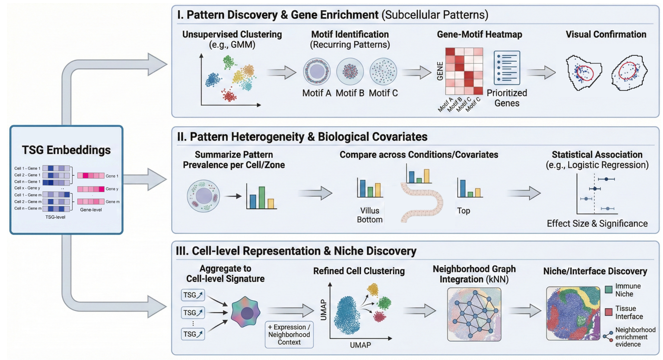
Downstream example I — Pattern discovery → gene enrichment (identify genes with clear subcellular patterns). TSG embeddings → unsupervised clustering (e.g., GMM; K chosen by elbow) → recurring localization motif clusters → visualize representative cells/TSGs per cluster to assign interpretable motif names → for each motif cluster, compute a gene-by-motif composition (fraction of a gene’s TSGs assigned to the motif) → generate gene-enrichment heatmaps and shortlist genes enriched in motifs of interest → visual confirmation in representative single-cell spot maps. Outputs: motif dictionary (cluster exemplars + labels), gene–motif enrichment table/heatmap, prioritized genes with representative examples.

Downstream example II — Pattern heterogeneity → association with biological covariates. Per-TSG motif labels (e.g., polar vs non-polar) → summarize per cell (or per zone) as pattern prevalence → compare prevalence across conditions/covariates (e.g., villus Bottom/Mid/Top; cycling vs non-cycling) → quantify effects using logistic regression with cell-clustered standard errors to account for repeated gene–cell measurements within cells. Outputs: effect sizes and significance for covariates, plots of prevalence across conditions, examples illustrating structured heterogeneity.

Downstream example III — Cell-level subcellular representation → refined clustering and niche/interface discovery. TSG embeddings → aggregate to cell-level subcellular signatures (pool across a cell’s gene–cell instances) → optionally concatenate with expression and/or neighborhood context → refined cell-state clustering (subcluster within a transcriptional group) → integrate with local neighborhood graphs (kNN) → identify niches/domains/interfaces supported by neighborhood enrichment (e.g., immune-neighbor fraction, adjacency probability). Outputs: refined subclusters, subcellular-augmented cell embeddings, niche/domain/interface labels with neighborhood enrichment evidence.