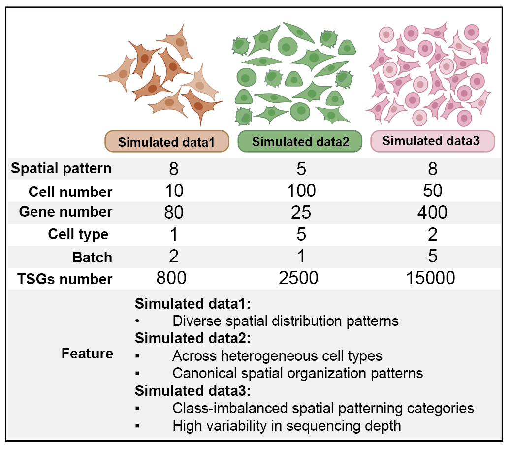
02_Simulated_datasets

1_dataset details

Dataset	Cell number	Gene number	Cell type	TSGs	Pattern	Ratio	Batch
Simulated_data1	10	80	1	800	8	5	2
Simulated_data2	100	25	5	2500	5	5	1
Simulated_data3	50	400	2	15000	8	10	5

Tips

• Using the built-in 318 cell templates from the simfish python package, 10/20 cells were randomly selected;- Generated RNA spatial localization data for 8 gene spatial distribution patterns: Random, Foci, Intranuclear, Extranuclear, Perinuclear, Pericellular, Protrusion, and Radial (ours);

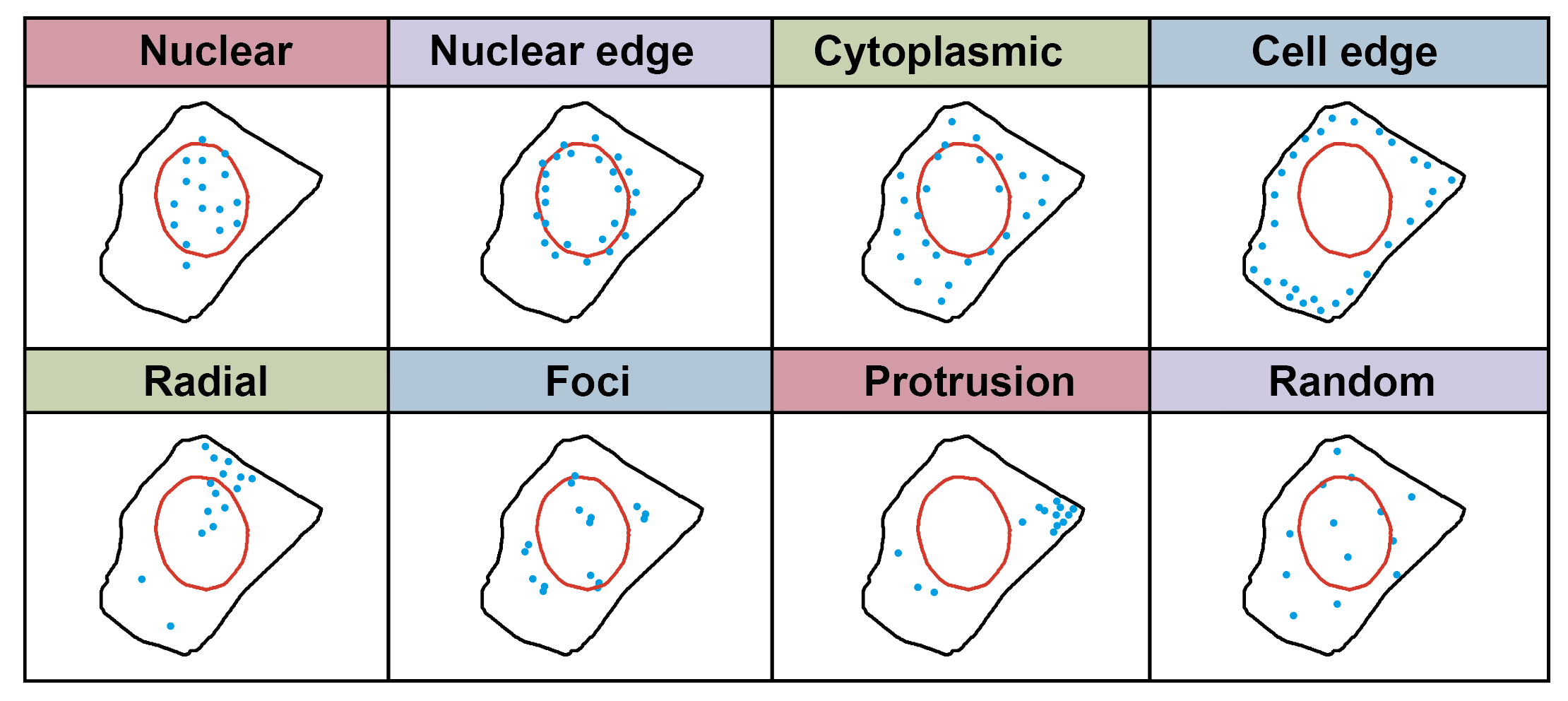
• Each spatial pattern simulated 5 different intensities of spatial distribution: 60%, 70%, 80%, 90%, and 100%, with higher intensity leading to more pronounced spatial distribution patterns;

• Each spatial pattern also simulated 25, 50, 100, 150, and 200 different transcript numbers;

• Different expression intensities and different transcript numbers of the same spatial pattern can be viewed as a gene expressing that pattern;

• Foci is a special pattern that does not require specification of transcript numbers.

2_GRASP preprocessing

step1: Load data

dataset = "simulated1"
outfile = f'../1_input/pkl_data/{dataset}_data_dict.pkl'

with open(outfile, 'rb') as f:
    pickle_dict = pickle.load(f)
    
df_registered = pickle_dict['df_registered'] 
cell_radii = pickle_dict['cell_radii']
cell_boundary = pickle_dict['cell_boundary']
nuclear_boundary = pickle_dict['nuclear_boundary']
nuclear_boundary_df_registered = pickle_dict['nuclear_boundary_df_registered'] 

step2: Visualize the original and normalized TSGs

path = "../2_scaled_cell"
cep.plot_raw_gene_distribution(dataset, cell_boundary, nuclear_boundary, df_registered, path)
cep.plot_register_gene_distribution(dataset, df_registered, path, nuclear_boundary_df_registered)

Processing cells: 100%|██████████| 10/10 [11:26<00:00, 68.62s/it]
All cell images have been saved to ../2_scaled_cell/simulated1/raw_gene/cell_cell_257
Plotting per cell: 100%|██████████| 10/10 [12:38<00:00, 75.84s/it]

step3: Cell partitioning

import utils_code.partition as pat

gene_list = df_registered['gene'].unique()
cell_list = df_registered['cell'].unique()
dir = f"../4_partition_same/{dataset}_partition/"
if not os.path.exists(dir):
    os.makedirs(dir)
for n_sectors in range(30, 31, 10):  
    for m_rings in range(15, 16, 5):   
        for target_cell in cell_list:    
            df = df_registered[df_registered['cell'] == target_cell]
            genes = df['gene'].unique()
            k_neighbor = int((n_sectors * m_rings) / 10) 
            plot_dir = os.path.join(dir,f"{target_cell}/{target_cell}_{n_sectors}_{m_rings}_k{k_neighbor}")
            if not os.path.exists(plot_dir):
                os.makedirs(plot_dir)
            print(f"This is [target_cell: {target_cell}] - [n_sectors: {n_sectors}] - [m_rings: {m_rings}], and k_neighbor is {k_neighbor}")                     
            nuclear_boundary_df = nuclear_boundary_df_registered[nuclear_boundary_df_registered['cell'] == target_cell]
            for gene in tqdm(gene_list, desc="Processing genes"): 
                df_filtered = df[df['gene'] == gene]
                r = 1  # r = cell_radii[target_cell]  
                count_matrix, center_points, point_counts, is_virtual, is_edge = pat.count_points_in_areas_same(df_filtered, n_sectors, m_rings, r) 
                nuclear_positions = pat.classify_center_points_with_edge(center_points, nuclear_boundary_df, is_edge) 
                edges = pat.build_graph_k_nearest(center_points, k=k_neighbor)
                G = pat.build_graph_with_networkx(center_points, edges, is_virtual)
                pat.save_node_data_to_csv_old(center_points, is_virtual, plot_dir, gene, point_counts, k=k_neighbor, nuclear_positions=nuclear_positions)
                pat.plot_cell_partition_heatmap(target_cell, gene, point_counts, n_sectors, m_rings, r, plot_dir, nuclear_boundary_df)

step4: Enhancement of TSGs

import utils_code.augumentation as aug

n_sectors = 30
m_rings = 15
k_neighbor = int((n_sectors * m_rings) / 10)
dropout_ratios = [0.1, 0.2, 0.3] 

dir = f"../4_partition_same/{dataset}_partition/"
gene_list = df_registered['gene'].unique()
cell_list = df_registered['cell'].unique()

for cell in tqdm(cell_list, desc="Processing all cells", leave=True):
    path = f"{dir}/{cell}/{cell}_{n_sectors}_{m_rings}_k{k_neighbor}"
    save_path = f"{dir}/{cell}/{cell}_{n_sectors}_{m_rings}_k{k_neighbor}_aug"
    if not os.path.exists(save_path):
        os.makedirs(save_path)
    for gene in tqdm(gene_list, desc="Processing all genes", leave=True):
        nodes_file = f'{path}/{gene}_node_matrix.csv'
        adj_file = f'{path}/{gene}_adj_matrix.csv'
        if not os.path.exists(nodes_file) or not os.path.exists(adj_file):
            print(f"Skipping {gene} in {cell} (file not found).")
            continue
        node_matrix = pd.read_csv(nodes_file)
        adj_matrix = pd.read_csv(adj_file)
        random_angle = random.uniform(0, 360)
        node_matrix_rotated = aug.rotate_nodes(node_matrix.copy(), random_angle)
        real_nodes_count = (node_matrix_rotated['is_virtual'] == 0).sum()
        if real_nodes_count >= 10:
            if real_nodes_count <= 100:
                dropout_ratio = dropout_ratios[0]
            elif real_nodes_count > 100 and real_nodes_count <= 150:
                dropout_ratio = dropout_ratios[1]
            else:
                dropout_ratio = dropout_ratios[2]
            # print(f"The gene {gene} needs to drop out {dropout_ratio}.")
            adj_matrix_dropped, node_matrix_dropped = aug.dropout_nodes(adj_matrix.copy(), node_matrix_rotated.copy(), dropout_ratio)
            adj_matrix_dropped.to_csv(f"{save_path}/{gene}_adj_matrix.csv", index=False)
            node_matrix_dropped.to_csv(f"{save_path}/{gene}_node_matrix.csv", index=False)
            # aug.plot_graph(adj_matrix, node_matrix,adj_matrix_dropped, node_matrix_dropped, f"{cell}_{gene}", save_path)
        else:
            # print(f"The gene {gene} not need to drop out.")
            adj_matrix.to_csv(f"{save_path}/{gene}_adj_matrix.csv", index=False)
            node_matrix_rotated.to_csv(f"{save_path}/{gene}_node_matrix.csv", index=False)
            # aug.plot_graph(adj_matrix, node_matrix, adj_matrix, node_matrix_rotated, f"{cell}_{gene}_original", save_path)
            

3_GRASP training

step5: Load all TSGs to prepare for training

cell_list = df_registered['cell'].unique()
gene_list = df_registered['gene'].unique()
cell_numbers = len(cell_list)
gene_numbers = len(gene_list)

n_sectors = 30
m_rings = 15
k_neighbor = int((n_sectors * m_rings) / 10)

path = f"../4_partition_same/{dataset}_partition" 
df = pd.read_csv(f"../1_input/label/{dataset}_label.csv")
original_graphs, augmented_graphs = gra.generate_graph_data_target(dataset, df, path, n_sectors, m_rings, k_neighbor)

print(len(original_graphs))
print(len(augmented_graphs))

gene_labels = [data.gene for data in original_graphs]
cell_labels = [data.cell for data in original_graphs]

Processing Graphs: 100%|██████████| 800/800 [3:22<00:00,  7.49it/s]  

graphs_number = len(original_graphs)
print(f"cell_numbers:{cell_numbers} - gene_numbers:{gene_numbers} - graphs_number:{graphs_number}")

save_path = f"../5_graph_data"
if not os.path.exists(save_path):
    os.makedirs(save_path)
graph_data = {"original_graphs": original_graphs, 
              "augmented_graphs": augmented_graphs,
              "gene_labels": gene_labels,
              "cell_labels": cell_labels}

save_file = f"{save_path}/{dataset}_cell{cell_numbers}_gene{gene_numbers}_graph{graphs_number}.pkl"
with open(save_file, 'wb') as f:  
    pickle.dump(graph_data, f)

print(f"Graph data saved to {save_file}")

cell_numbers:10 - gene_numbers:80 - graphs_number:800
Graph data saved to ../5_graph_data/simulated1_cell10_gene80_graph800.pkl

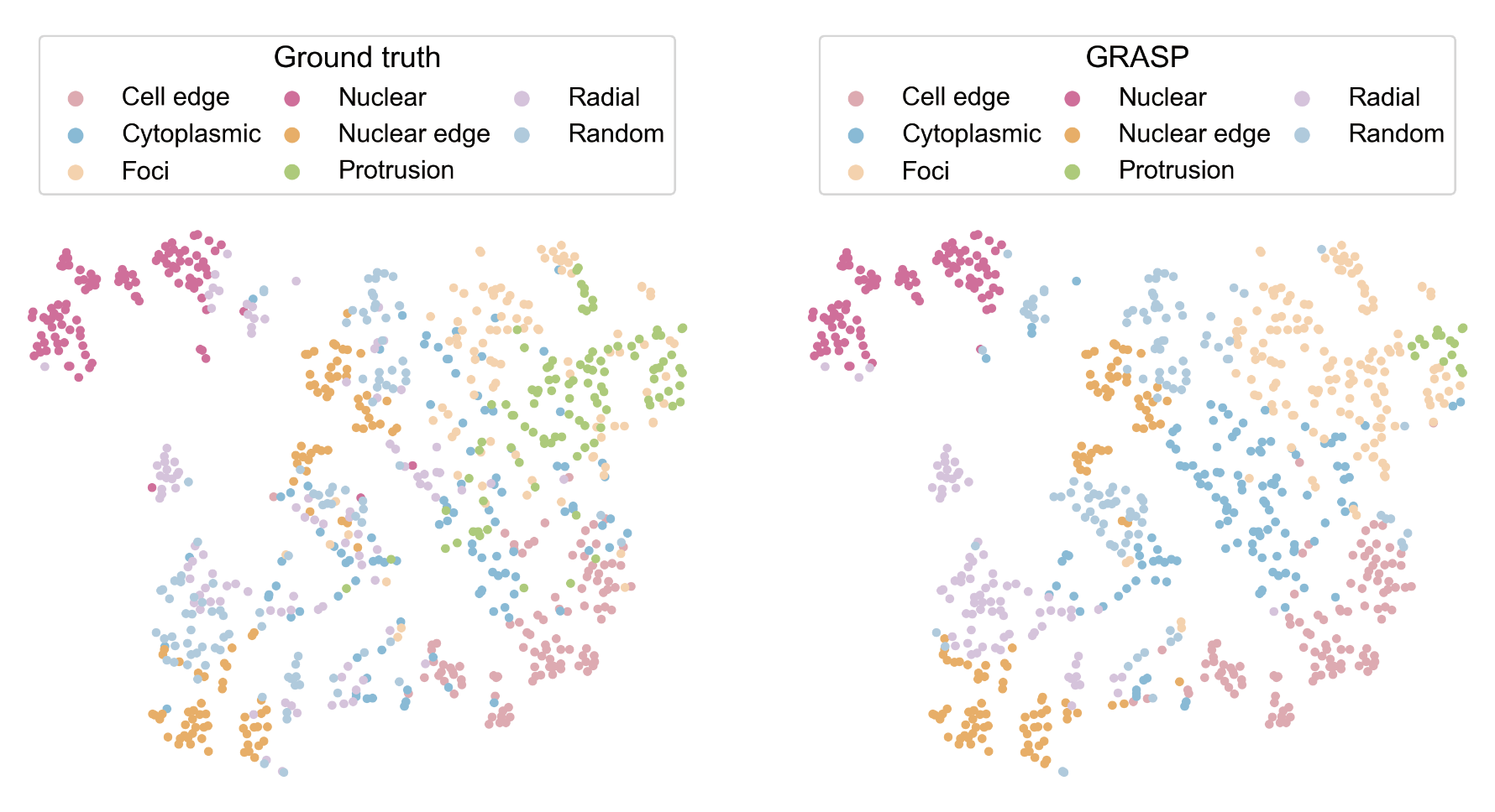
step6: Clustering and identifying spatial localization patterns

a, b = 0.4, 0.6 
dataset = "simulated1"
path1 = f'../1.5_benchmark/figure/{dataset}/s1_tsne_ours_a{a}_b{b}'
path2 = f'../1.5_benchmark/figure/{dataset}/s1_tsne_gt_a{a}_b{b}'

ours_label = pd.read_csv(f"../1.5_benchmark/method4_ours/{dataset}/ours_label_a{a}_b{b}.csv")
ours_label['pattern'].value_counts()

# 定义 color_map
color_map = {'Nuclear': '#ed6ca4', 'Cytoplasmic': '#7bc4e2', 'Protrusion': '#acd372', 'Nuclear edge':'#fbb05b',
             'Cell edge': '#EDABB5', 'Random':'#ACD0E4', 'Foci':'#FFD4AB', 'Radial':'#DDC4E0'}

plot_tsne_by_label(df=ours_label,label_col='pattern',color_map=color_map, title='', save_prefix=path1,
    legend_title='GRASP', legend_loc='upper left', legend_bbox=(0.5, 1), legend_ncol=3)

plot_tsne_by_label(df=ours_label, label_col='groundtruth', color_map=color_map, title='', save_prefix=path2,
    legend_title='Ground truth', legend_loc='upper left', legend_bbox=(0.5, 1.0), legend_ncol=3)